📈 Visualizing High-Dimensional Data
(Parallel Coordinates · Deviation Chart · Andrews Curve)
1️⃣ Introduction
When data has more than three dimensions, standard 2D or 3D plots fail to reveal structure.
We use specialized projection and transformation techniques to visualize multivariate patterns:
-
Parallel Coordinate Plots (PCP) — visualize multi-attribute records as lines.
-
Deviation Charts — highlight differences from a baseline (useful for comparisons).
-
Andrews Curves — map multivariate points to continuous periodic functions.
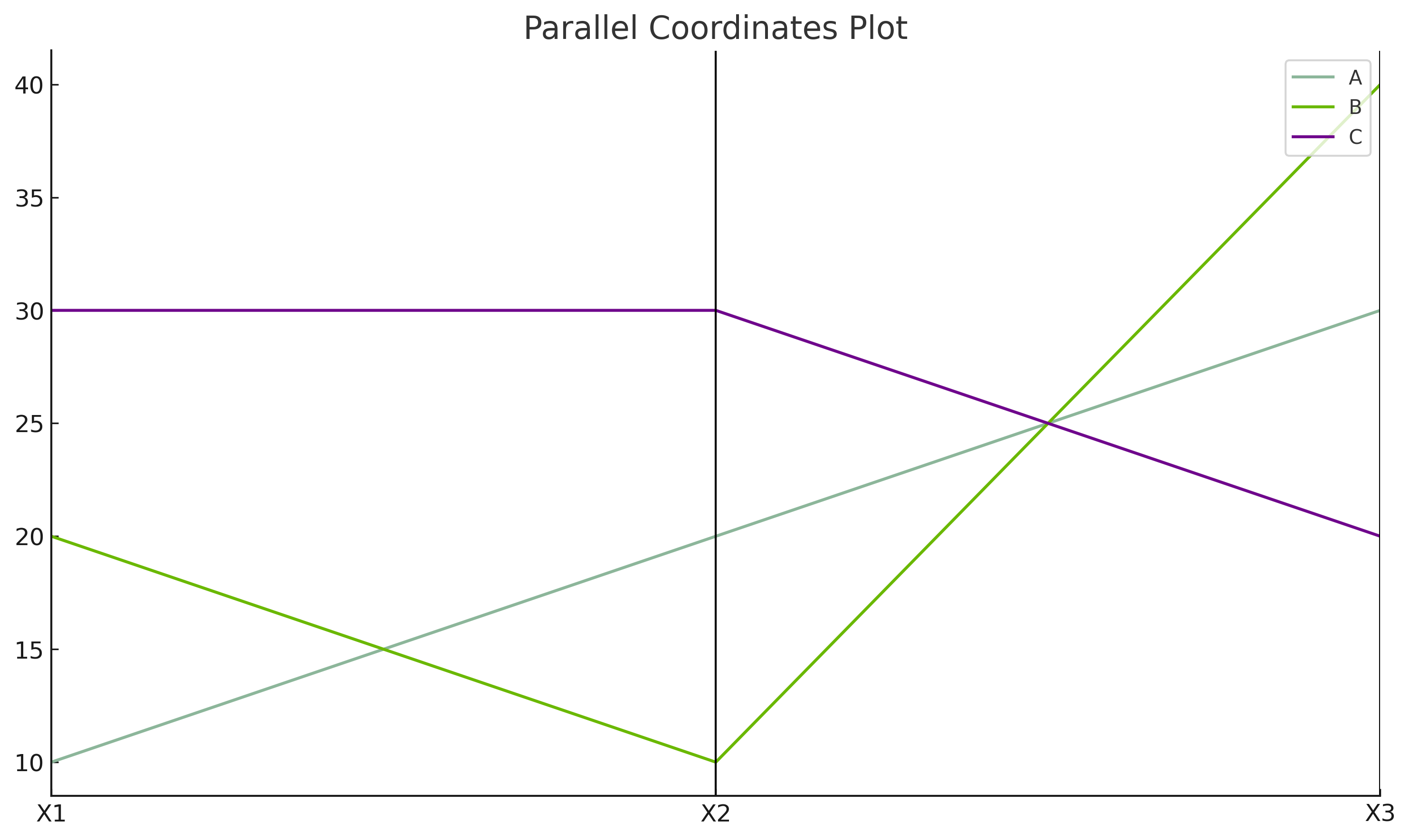
2️⃣ Parallel Coordinate Chart (PCP)
Theory
Given \(p\) variables \(( x_1, x_2, ..., x_p )\), each record \(( i )\) is a vector
\((\mathbf{x}^{(i)} = (x^{(i)}_1, x^{(i)}_2, \dots, x^{(i)}_p))\) Each variable is drawn on a parallel axis.
Each record is plotted as a polyline connecting values across axes.
Mathematical Normalization
\((x'_{ij} = \dfrac{x_{ij} - \min(x_j)}{\max(x_j) - \min(x_j)})\)
Manual Example
Original data and normalized values (min=10, max=30 for all three variables):
| Observation | X1 | X2 | X3 |
|---|---|---|---|
| A | 10 | 20 | 30 |
| B | 20 | 10 | 40 |
| C | 30 | 30 | 20 |
Normalized: \((x'_{ij}=(x_{ij}-10)/(30-10))\)
| Observation | X1' | X2' | X3' |
|---|---|---|---|
| A | 0.0 | 0.5 | 0.5 |
| B | 0.5 | 0.0 | 1.0 |
| C | 1.0 | 1.0 | 0.0 |
Example Figure
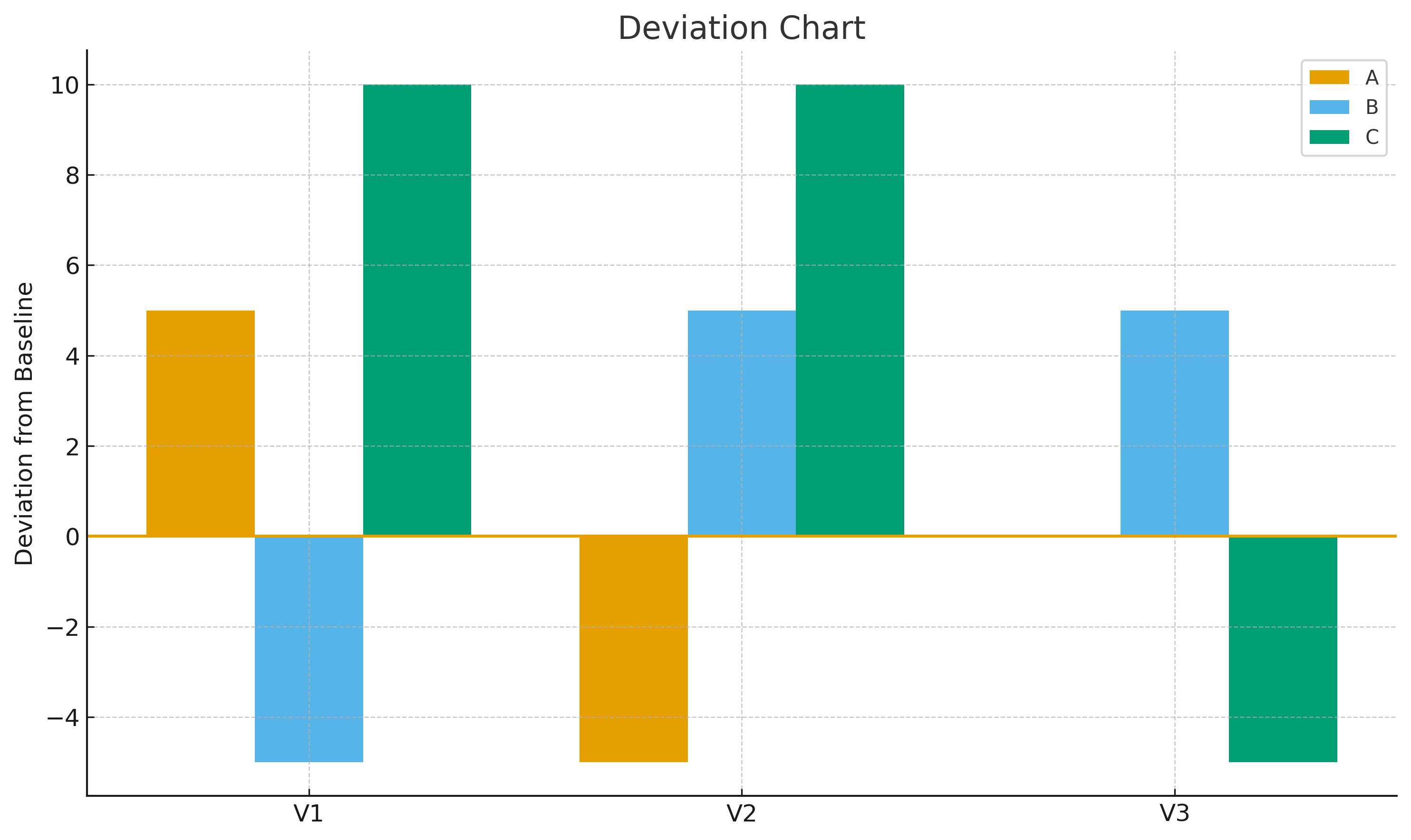
3️⃣ Deviation Chart
Theory
A Deviation Chart displays differences from a baseline \(( b_j )\) for each variable \(( j )\):
\(( d_{ij} = x_{ij} - b_j )\)
Manual Example
Baseline \((b=[50,30,20])\). Observations:
- A = [55, 25, 20] → \((d_A=[+5,-5,0])\)
- B = [45, 35, 25] → \((d_B=[-5,+5,+5])\)
- C = [60, 40, 15] → \((d_C=[+10,+10,-5])\)
Example Figure
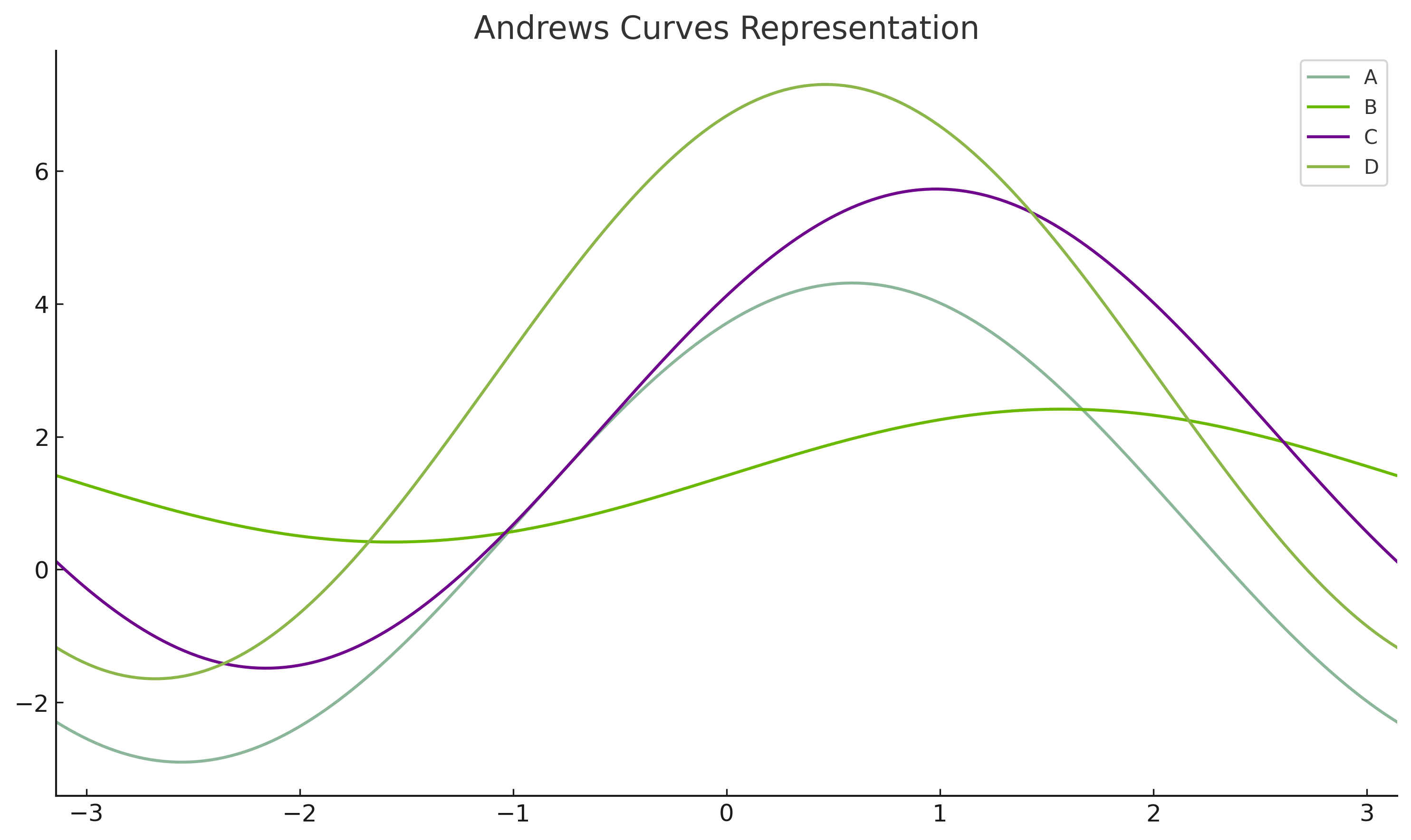
4️⃣ Andrews Curves
Theory
Each data point in \((\mathbb{R}^p)\) is represented by
with \((t\in[-\pi,\pi])\). Curve similarity reflects data similarity.
Manual Example (3 features)
For A(1,2,3) and B(2,1,0): $$ f_A(t) = 1/\sqrt{2} + 2\sin t + 3\cos t,\; f_B(t) = 2/\sqrt{2} + \sin t. $$ Evaluate at \((t=0,\pi/2,\pi)\) to compare values and shapes.
Example Figure
5️⃣ Practice Problems (By Hand)
- PCP: Normalize and sketch lines for A(1,2,3,4), B(4,3,2,1), C(2,2,2,2). Identify negatively correlated pairs.
- Deviation: With baseline [10,20,30], compute deviations for P(12,18,33), Q(9,21,27) and interpret.
- Andrews: Compute \((f(t))\) for x=(1,0,2) at \((t=0,\pi/2,\pi)\) and compare with y=(2,1,1).