Chapter 6 - Statistical Methods
1. Histogram¶
✳️ Definition¶
A histogram shows frequency distribution of data grouped into bins.
🧮 Formula
Frequency in bin 𝑖
\( f_𝑖 \) = Number of observations in bin 𝑖
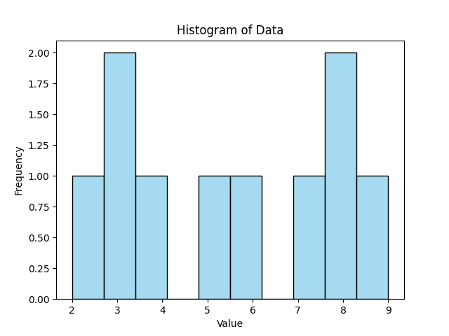
🧮 Manual Example¶
Data: [2, 3, 3, 4, 5, 6, 7, 8, 8, 9]
Bin width = 2
Bins: (2–4), (4–6), (6–8), (8–10)
| Bin | Frequency |
|---|---|
| 2–4 | 3 |
| 4–6 | 2 |
| 6–8 | 3 |
| 8–10 | 2 |
Plot bars with heights as frequencies.
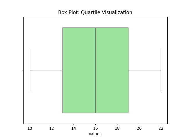
2. Box Plot (Quartile Visualization)¶
✳️ Definition¶
A box plot summarizes data based on five-number summary:
🧮 Manual Example¶
Draw box from Q1–Q3, line at Median, whiskers to min & max.
<
3. Distribution Chart (KDE Plot)¶
✳️ Definition¶
A KDE plot estimates probability density by smoothing the histogram.
i) What is KDE?¶
Given a univariate sample \((x_1,\dots,x_n)\), the KDE at a point \((x)\) is
where: - \((K(\cdot))\) is a kernel (e.g., Gaussian, Epanechnikov, Uniform, Triangular), \((\int K(u)\,du=1)\),
- \((h>0)\) is the bandwidth (smoothing parameter).
Intuition. Each observation contributes a small “bump” centered at \((x_i)\); the final curve is their average. Smaller \((h)\) → more wiggly; larger \((h)\) → smoother.
ii) Common Kernels (closed forms)¶
-
Gaussian: \((K(u)=\dfrac{1}{\sqrt{2\pi}}e^{-u^2/2})\)
-
Epanechnikov: \((K(u)=\dfrac{3}{4}(1-u^2)\mathbf{1}\{|u|\le 1\})\)
-
Uniform (Rectangular): \((K(u)=\dfrac12\mathbf{1}\{|u|\le 1\})\)
-
Triangular: \((K(u)=(1-|u|)\mathbf{1}\{|u|\le 1\})\)
In practice, the bandwidth matters more than the specific kernel choice for smooth densities.
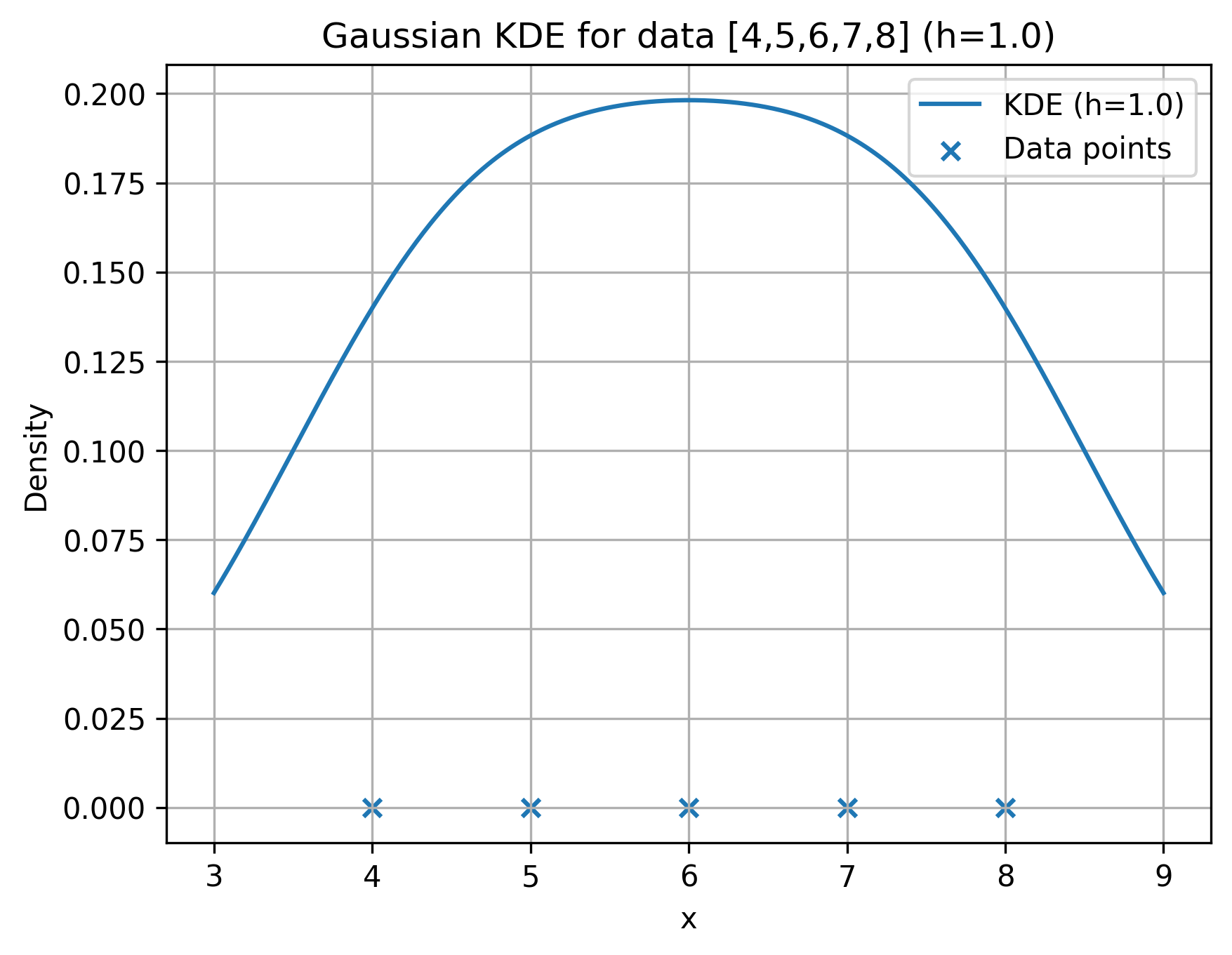
iii) Manual Example A — Gaussian kernel, explicit numbers¶
Dataset: \((x=\{4,5,6,7,8\})\) (so \((n=5)\)).
Useful Gaussian values (to 6 d.p.): \(\phi(0)=0.398942,\phi(0.5)=0.352065,\phi(1)=0.241971\)
\(\phi(1.5)=0.129518,\phi(2)=0.053991,\phi(2.5)=0.017528\)
\(\phi(3)=0.004432,\phi(4)=0.000134.\)
A1) KDE at \((x=6)\) with bandwidth \((h=1)\)¶
Standardized offsets \((u_i=(x- x_i)/h)\): \(((2,1,0,-1,-2))\).
Contributions: \((\phi(2),\phi(1),\phi(0),\phi(1),\phi(2))\).
\(\sum \phi = 0.053991 + 0.241971 + 0.398942 + 0.241971 + 0.053991 = 0.990866.\)
\(\hat f_{h=1}(6) = \frac{1}{n h}\sum \phi = \frac{0.990866}{5\cdot 1} = \boxed{0.198173}.\)
A2) KDE at \((x=5)\) with \((h=1)\)¶
Offsets \((u=(1,0,-1,-2,-3))\) → \((\phi(1)+\phi(0)+\phi(1)+\phi(2)+\phi(3))\).
\(\sum \phi = 0.241971 + 0.398942 + 0.241971 + 0.053991 + 0.004432 = 0.941307.\)
\(\hat f_{h=1}(5) = \frac{0.941307}{5} = \boxed{0.188261}.\)
A3) Effect of bandwidth at \((x=6)\)¶
- \((h=0.5)\): \((u=(4,2,0,-2,-4))\) → \((\phi(4)+\phi(2)+\phi(0)+\phi(2)+\phi(4))\)
\((\sum \phi = 0.000134 + 0.053991 + 0.398942 + 0.053991 + 0.000134 = 0.507192)\).
\((\hat f = \dfrac{1}{n h}\sum = \dfrac{0.507192}{5\cdot 0.5} = \boxed{0.202877})\).
- \((h=2)\): \((u=(1,0.5,0,-0.5,-1))\) → \((\phi(1)+\phi(0.5)+\phi(0)+\phi(0.5)+\phi(1))\)
\((\sum \phi = 0.241971 + 0.352065 + 0.398942 + 0.352065 + 0.241971 = 1.587014)\).
\((\hat f = \dfrac{1.587014}{5\cdot 2} = \boxed{0.158701})\).
Observation. Increasing \((h)\) lowered the peak (more smoothing). Decreasing \((h)\) raised the peak/sharpness.
iv) Manual Example B — Epanechnikov kernel, \((h=1)\)¶
At \((x=6)\): \((u=(2,1,0,-1,-2))\). Only \((|u|\le 1)\) contribute: \((u=1,0,-1)\).
\((K(1)=0,\;K(0)=\tfrac34,\;K(-1)=0)\).
\(\sum K = 0 + 0.75 + 0 = 0.75,\quad \hat f = \frac{0.75}{n h} = \frac{0.75}{5\cdot 1} = \boxed{0.15}.\)
v) Choosing Bandwidth by Hand (closed‑form rules)¶
Let \((s)\) be sample standard deviation; \((\text{IQR}=Q_3-Q_1)\).
Define \((n^{-1/5})\) (for \((n=5)\), \((n^{-1/5}\approx 0.72478)\)).
-
Scott’s rule (Normal reference): \(h_{\text{Scott}} = 1.06\, s\, n^{-1/5}.\)
-
Silverman’s rule of thumb: \(h_{\text{Silv}} = 0.9\;\min\!\left(s, \frac{\text{IQR}}{1.34}\right)\! n^{-1/5}.\)
For our dataset \( x=\{4,5,6,7,8\} \):
- Mean \(=6 \). Using sample SD: \((s=\sqrt{\tfrac{\sum(x_i-6)^2}{n-1}}=\sqrt{\tfrac{10}{4}}=1.58114)\)
-
Quartiles (hinges): \((Q_1\approx 5,\; Q_3\approx 7 \Rightarrow \text{IQR}=2)\), \((\text{IQR}/1.34=1.49254)\).
-
\((n^{-1/5}\approx 0.72478)\).
Hence, \(h_{\text{Scott}} \approx 1.06\times 1.58114 \times 0.72478 = \boxed{1.215},\)
\(h_{\text{Silv}} \approx 0.9\times \min(1.58114,\,1.49254)\times 0.72478 = 0.9\times 1.49254 \times 0.72478 \approx \boxed{0.973}.\)
vi) Hand‑Computation Template (exam‑ready)¶
Input: sample \((x_1,\dots,x_n)\), kernel \((K)\), bandwidth \((h)\), target evaluation point \((x^\star)\).
Steps:
1. Compute offsets \((u_i=\dfrac{x^\star - x_i}{h})\).
-
For each \((u_i)\), evaluate \((K(u_i))\) (using table/known values).
-
Sum: \((S=\sum_{i=1}^n K(u_i))\).
-
Output: \((\hat f(x^\star)=\dfrac{S}{n h})\).
-
Repeat for a grid of \((x^\star)\) to sketch the curve by hand.
vii) Worked Mini‑Grid (Gaussian, \((h=1)\))¶
Dataset as before. Evaluate \((\hat f(x))\) at \((x=\{5,6,7\})\).
Because of symmetry, \((\hat f(5)=\hat f(7))\).
| \((x)\) | Offsets \((u)\) for \((\{4,5,6,7,8\})\) | Sum of \((\phi(u))\) | \((\hat f(x)=\dfrac{1}{5}\sum \phi(u))\) |
|---|---|---|---|
| 5 | (1,0,-1,-2,-3) | 0.941307 | 0.188261 |
| 6 | (2,1,0,-1,-2) | 0.990866 | 0.198173 |
| 7 | (3,2,1,0,-1) | 0.941307 | 0.188261 |
viii) Comparing KDE vs Histogram (manual)¶
Same data, bins of width 2: (2–4], (4–6], (6–8], (8–10]
Frequencies: 0, 2, 3, 0 → bars at 0, 2, 3, 0.
KDE is smooth and does not depend on bin edges; histogram does.
ix) Boundary Bias & Discrete Data¶
- For supports like \(([0,\infty))\), Gaussian kernels “spill” mass into negatives near 0. Fixes: boundary‑corrected kernels, reflection, or transformation (e.g., log).
- KDE assumes continuous data; for discrete/integer data, consider jittering or discrete kernels.
x) Multimodality by Hand (quick check)¶
If data cluster near two centers, KDE will show two peaks when \((h)\) is small enough to resolve them. Try two clusters (e.g., \((\{0,0.2,0.1\}\cup\{3,3.1,3.2\})\)) and compute at midpoints to see valley between modes.
xi) Short Exam Problems (with answers)¶
Q1. For \((x=\{4,5,6,7,8\})\), Gaussian kernel, \((h=1)\), compute \((\hat f(6))\).
A. \((0.1982)\) (from §3 A1).
Q2. Same data, Epanechnikov, \((h=1)\), compute \((\hat f(6))\).
A. \((0.15)\) (from §4).
Q3. Using Silverman’s rule, approximate \((h)\).
A. \((\approx 0.973)\) (from §5).
Q4. Explain effect of doubling \((h)\) on the KDE at a peak.
A. Peak height typically decreases; curve becomes smoother (see §3 A3).
xii) Quick Reference Values (Gaussian \((\phi(u))\))¶
\(\small\begin{array}{c|cccccccc} u & 0 & 0.5 & 1 & 1.5 & 2 & 2.5 & 3 & 4\\\hline \phi(u) & 0.399 & 0.352 & 0.242 & 0.130 & 0.054 & 0.018 & 0.004 & 0.0001 \end{array}\)
Summary Table¶
| Visualization | Purpose | Manual Computation |
|---|---|---|
| Quantile Plot | Plot cumulative probabilities | (i-0.5)/n vs x(i) |
| Q–Q Plot | Compare data quantiles to theoretical | z-scores vs data |
| Histogram | Frequency count | Bin width, frequencies |
| Box Plot | Quartile-based summary | Min, Q1, Median, Q3, Max |
| KDE Plot | Smooth probability density | Kernel formula |
🧩 References¶
- Tukey, J. W. (1977). Exploratory Data Analysis. Addison-Wesley.
- Cleveland, W. S. (1993). Visualizing Data. Hobart Press.
- Seaborn Documentation: https://seaborn.pydata.org
- Matplotlib Documentation: https://matplotlib.org