📘 Chapter 14 — Regression¶

Goal: Understand Linear Regression and Logistic Regression (for classification), and master core regression metrics: MAE, MSE, RMSE, R². Includes theory, math, by-hand examples.

1) Linear Regression¶

1.1 Problem Setup¶

Given data points $(x_i, y_i)$ for $i=1,\dots,n$, fit a line $$ \hat y_i = \beta_0 + \beta_1 x_i $$ that minimizes the sum of squared errors (SSE): $$ \text{SSE}(\beta_0,\beta_1) = \sum_{i=1}^n (y_i - \beta_0 - \beta_1 x_i)^2 . $$

1.2 Closed-Form (Normal Equations)¶

Let $\bar x$ and $\bar y$ be sample means. $$ \hat\beta_1 = \frac{\sum_i (x_i-\bar x)(y_i-\bar y)}{\sum_i (x_i-\bar x)^2}, \qquad \hat\beta_0 = \bar y - \hat\beta_1 \bar x . $$

Matrix form: with $X = [\,x\ \ 1\,]$ and $y \in \mathbb{R}^n$, $$ \hat{\boldsymbol\beta} = (X^\top X)^{-1} X^\top y,\quad \boldsymbol\beta = \begin{bmatrix}\beta_1\ \beta_0\end{bmatrix}. $$

1.3 By-Hand Example (tiny dataset)¶

Data: $(x,y) \in \{(1,2),(2,3),(3,5),(4,4),(5,7)\}$.
Compute means: $\bar x=3,\ \bar y=4.2$.

$\sum (x-\bar x)(y-\bar y) = 11.0$ and $\sum (x-\bar x)^2=10$.
So $\hat\beta_1 = 11/10 = 1.1$.
$\hat\beta_0 = 4.2 - 1.1\cdot 3 = 0.9$.
Fitted line: $\hat y = 0.9 + 1.1x$.

Now compute predictions and residuals:

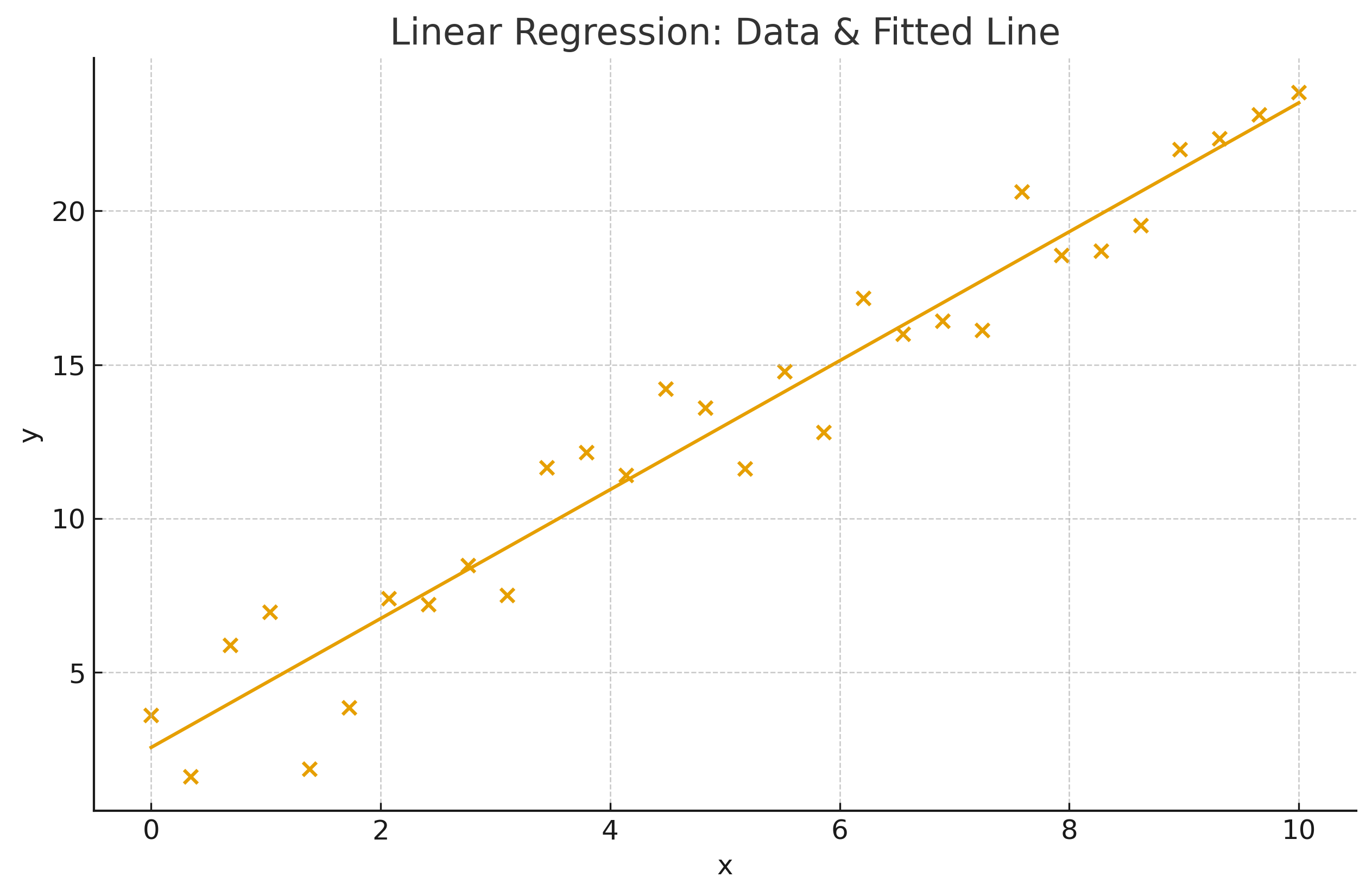
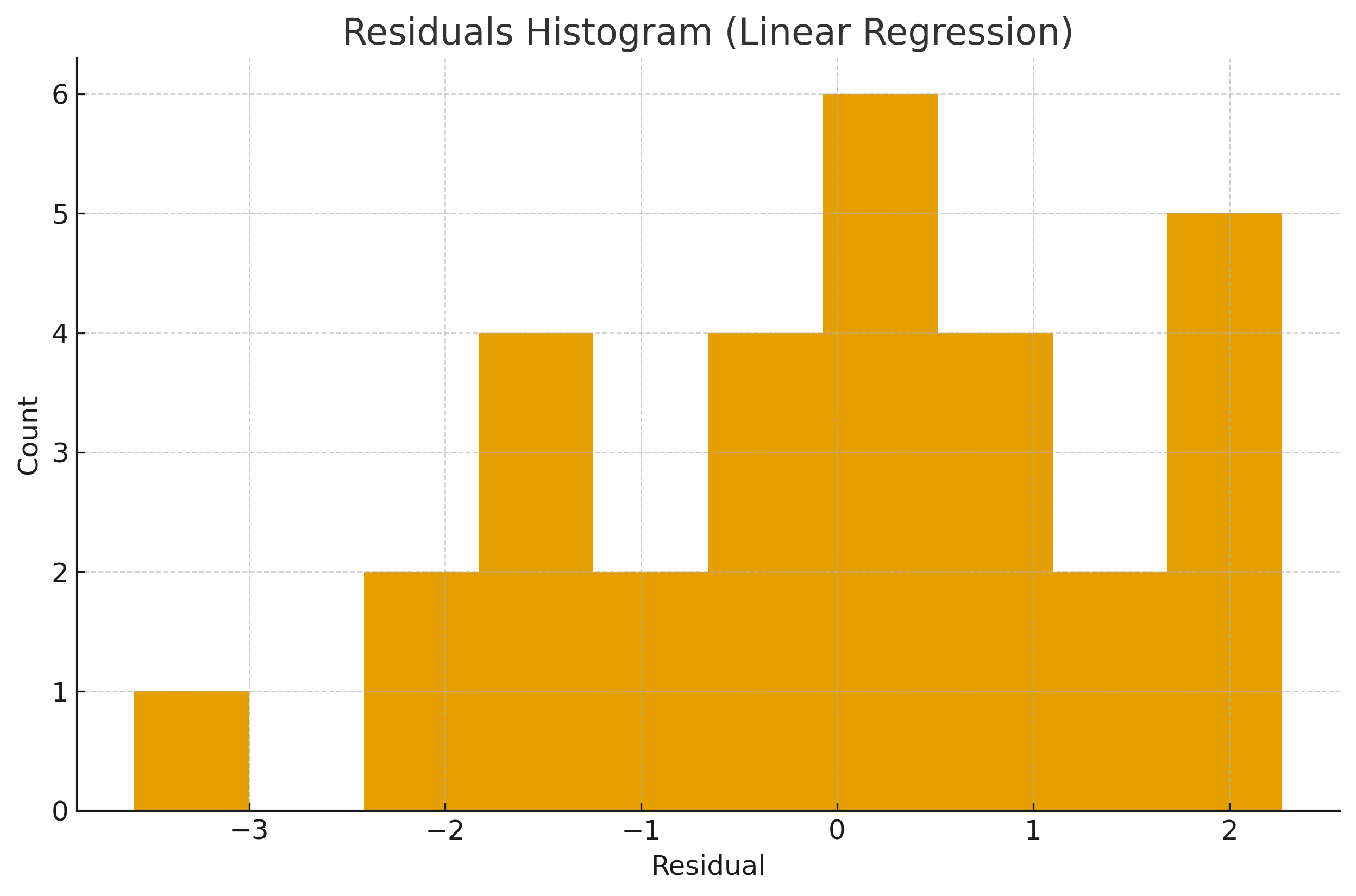
\[ \begin{array}{c|ccccc} x & 1 & 2 & 3 & 4 & 5 \\\hline y & 2 & 3 & 5 & 4 & 7 \\ \hat y & 2.0 & 3.1 & 4.2 & 5.3 & 6.4 \\ e=y-\hat y & 0.0 & -0.1 & 0.8 & -1.3 & 0.6 \end{array} \]

1.4 Visuals¶

Linear Regression: Data & Fitted Line

Residuals Histogram (Linear Regression)

2) Logistic Regression (for Classification)¶

2.1 Model¶

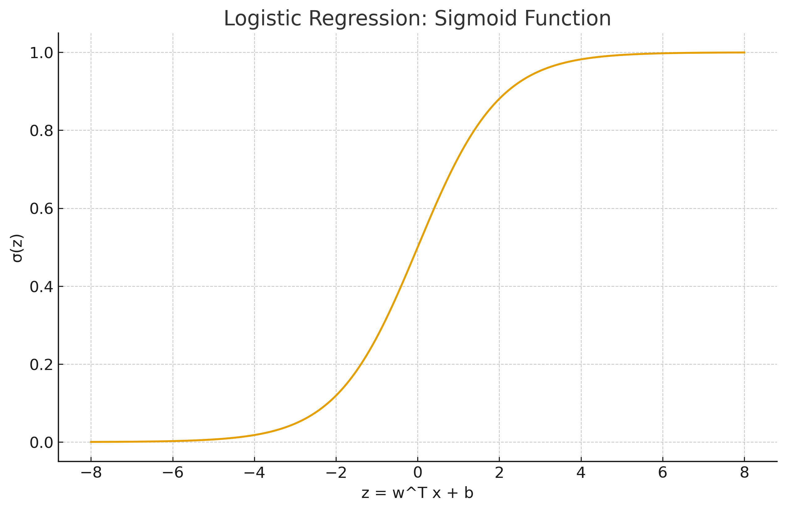
For binary $y\in\{0,1\}$, logistic regression models the log-odds via a linear function: $$ \log\frac{p(y=1\mid \mathbf x)}{1-p(y=1\mid \mathbf x)} = \mathbf w^\top \mathbf x + b, $$ so that $$ p(y=1\mid \mathbf x) = \sigma(\mathbf w^\top \mathbf x + b) = \frac{1}{1+e^{-(\mathbf w^\top \mathbf x + b)}} . $$ Decision rule (default): predict $1$ if $p \ge 0.5$, else $0$.

2.2 Maximum Likelihood & Loss¶

Given data $\{(\mathbf x_i,y_i)\}$, the (negative) log-likelihood $$ \mathcal L(\mathbf w,b)= -\sum_{i=1}^n \Big[y_i\log \sigma(z_i) + (1-y_i)\log(1-\sigma(z_i))\Big],\quad z_i=\mathbf w^\top \mathbf x_i + b. $$ Minimize $\mathcal L$ using gradient-based optimization.

2.3 Visual¶

Logistic Regression: Sigmoid Function

3) Regression Metrics¶

Given true values $y_i$ and predictions $\hat y_i$:

3.1 Mean Absolute Error (MAE)¶

\[ \text{MAE} = \frac{1}{n}\sum_{i=1}^n |y_i - \hat y_i| . \]

3.2 Mean Squared Error (MSE)¶

\[ \text{MSE} = \frac{1}{n}\sum_{i=1}^n (y_i - \hat y_i)^2 . \]

3.3 Root Mean Squared Error (RMSE)¶

\[ \text{RMSE} = \sqrt{\text{MSE}} . \]

3.4 Coefficient of Determination (R²)¶

Let $\bar y=\frac{1}{n}\sum_i y_i$.

Define $\text{SS}_{{tot}}=\sum_i (y_i-\bar y)^2$ and $\text{SS}_{{res}}=\sum_i (y_i-\hat y_i)^2$.

\[ R^2 = 1 - \frac{\text{SS}_{{res}}}{\text{SS}_{{tot}}} . \]

3.5 By-Hand Metric Example¶

Using the tiny dataset and the fitted line $\hat y=0.9+1.1x$: $\begin{array}{c|ccccc} x & 1 & 2 & 3 & 4 & 5 \\ \hline y & 2 & 3 & 5 & 4 & 7 \\ \hat y & 2.0 & 3.1 & 4.2 & 5.3 & 6.4 \\ |e| & 0.0 & 0.1 & 0.8 & 1.3 & 0.6 \\ e^2 & 0.0 & 0.01 & 0.64 & 1.69 & 0.36 \end{array}$

$\text{MAE}=(0+0.1+0.8+1.3+0.6)/5=0.56$.
$\text{MSE}=(0+0.01+0.64+1.69+0.36)/5=0.54$.
$\text{RMSE}=\sqrt{0.54}=0.735$.
$\bar y=4.2\Rightarrow \text{SS}_{{tot}}=14.8$, $\text{SS}_{{res}}=5\cdot 0.54=2.7$.
$R^2=1-2.7/14.8=0.8189$ (≈ 0.819).

4) Practice Questions¶

Derive the OLS solution $(X^\top X)^{-1}X^\top y$ starting from SSE.
Why is logistic regression optimized by maximum likelihood rather than least squares?
Show that minimizing MSE is equivalent to maximizing the Gaussian likelihood (with fixed variance).
Given $\text{SS}_{{tot}}=100$ and $\text{SS}_{{res}}=35$, compute $R^2$.
For the by-hand dataset, recompute MAE/MSE/RMSE if the model is $\hat y=1+1.0x$.